

From LinkedIn’s internal tool to the de facto standard for event streaming, how Kafka changed the way we think about data in motion.
Every time you get a fraud alert from your bank, see a “your order shipped” notification, or watch Netflix adapt its recommendation engine within seconds of your last watch, Apache Kafka is almost certainly involved. It’s become the invisible plumbing of the modern internet and for good reason.
In this guide, we’ll peel back the layers of Kafka’s architecture, understand why it outperforms traditional message queues at scale, and see exactly where and how it fits into production data stacks today.

What is Apache Kafka — and why does it matter?
Apache Kafka is a distributed event streaming platform built for high-throughput, fault-tolerant, and low-latency data pipelines. Originally created at LinkedIn in 2011 to handle activity stream data and operational metrics, it was open-sourced and donated to the Apache Software Foundation in 2012.
At its core, Kafka is not just a message queue. It’s a distributed commit log, an append-only, ordered, persistent stream of events that any number of consumers can read, at any time, at their own pace.
This seemingly simple distinction, a durable, replayable log versus a consumed-and-discarded queue, is what makes Kafka so uniquely powerful in data-intensive architectures.
Kafka’s core architecture
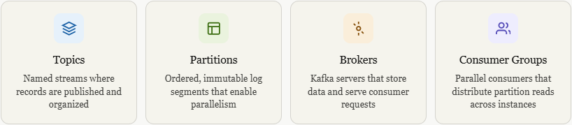
Each topic in Kafka is split into one or more partitions. Messages in a partition are strictly ordered and assigned an offset, a monotonically increasing integer that consumers track to know where they left off. This design is what enables Kafka’s legendary horizontal scalability.
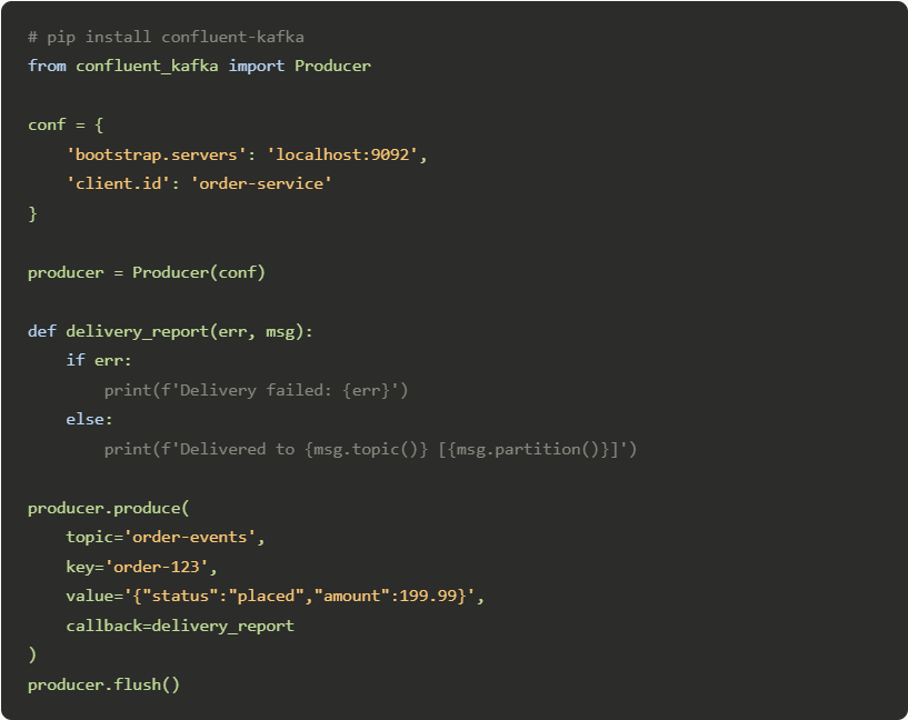
A producer in 15 lines of Python: —
Kafka vs. traditional message queues
If you’ve worked with RabbitMQ, ActiveMQ, or AWS SQS, you might wonder: “Aren’t they all just message queues?” Not quite. Here’s the critical distinction: traditional queues delete a message once it’s consumed. Kafka retains it for a configurable retention period (days, weeks, or indefinitely), and any number of consumers can read the same message independently.
This enables entirely new patterns like event sourcing, audit logs, and replaying historical events into new microservices, impossible in a classical queue model.
Real-world use cases across industries
Real-time fraud detection: — Banks stream transaction events through Kafka to ML scoring services that flag anomalies within milliseconds of a swipe.
Microservices decoupling: Services publish events instead of making direct API calls, removing tight coupling and enabling independent deployment.
Log aggregation: Application logs from thousands of servers are funnelled into Kafka and forwarded to Elasticsearch or S3 for centralized analysis.
Change Data Capture: Kafka Connect with Debezium captures every database row change and propagates it to downstream consumers in real time.
IoT data ingestion: Billions of device telemetry points per day like smart meters, factory sensors, connected cars, land in Kafka before analytics.
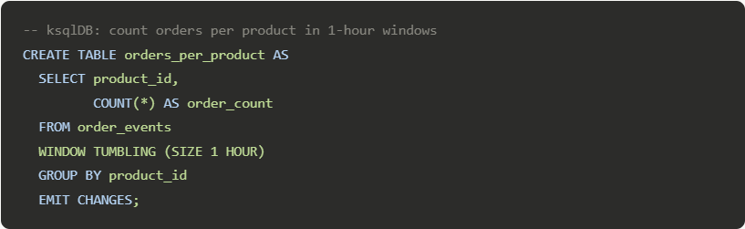
Stream processing: Kafka Streams and ksqlDB allow stateful computations, aggregations, joins, windowing directly on the data stream.
Kafka Streams vs ksqlDB — which should you use?
Both tools let you process events in motion, but they serve different audiences. Kafka Streams is a Java/Scala library embedded in your application, perfect for developers who want full programmatic control. ksqlDB exposes a SQL-like interface for defining stream transformations declaratively, making it accessible to data analysts and teams that prefer SQL over Java.
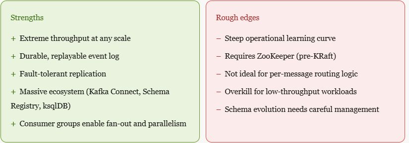
Kafka’s strengths and rough edges
KRaft mode — Kafka without ZooKeeper
One of the most significant architectural shifts in Kafka’s recent history is the removal of Apache ZooKeeper as an external dependency. The KRaft (Kafka Raft Metadata) mode, introduced experimentally in Kafka 2.8 and production-ready since 3.3, replaces ZooKeeper with a self-managed quorum of controller brokers using the Raft consensus algorithm.
This simplifies cluster operations dramatically, fewer moving parts, simpler deployment, better startup times, and support for millions of partitions per cluster (compared to tens of thousands in ZooKeeper mode). If you’re starting a new Kafka deployment today, KRaft is the way to go.
Getting started: should you self-host or go managed?
Self-hosting Kafka gives you complete control but demands real operational expertise like JVM tuning, replication configuration, disk management, and monitoring. For most teams, a managed offering is the pragmatic starting point:
Confluent Cloud is the most feature-complete managed Kafka, built by Kafka’s original creators. Amazon MSK is tightly integrated with the AWS ecosystem. Redpanda is a Kafka-compatible alternative written in C++ that eliminates the JVM entirely and offers impressive performance on smaller hardware.
Rule of thumb: if your team doesn’t yet have Kafka expertise, use a managed service. When throughput costs exceed $1,000/month or you need custom broker tuning, then evaluate self-hosting.
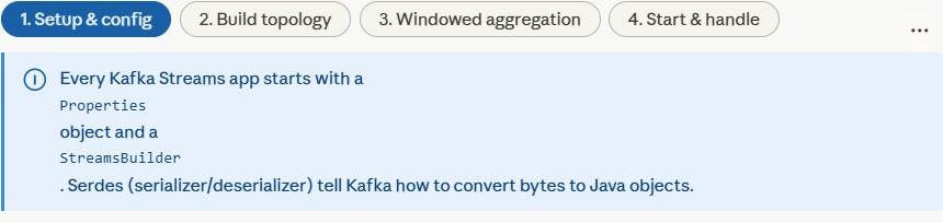
Kafka Streams
Kafka Streams is a client library built directly into Apache Kafka that lets you write real-time stream processing applications using plain Java/Scala, no separate cluster needed.
The core idea: Your app reads from one or more Kafka topics, applies transformations (filter, map, aggregate, join), and writes results back to another Kafka topic. The processing happens continuously as records arrive.
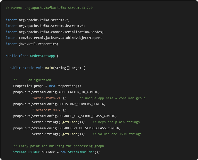
Pipeline for a real-time order analytics engine:

Now here’s the complete working Java implementation of that exact topology, with annotations explaining each step:
KStream: Unbounded event log — Every record is an independent event. Same key can appear many times. Good for: transactions, clicks, logs.
KTable: Changelog / latest value — Each key has exactly one current value. New records overwrite old. Good for: user profiles, inventory counts.
Tumbling window: Fixed, non-overlapping buckets — Events fall into exactly one 1-min bucket. No overlap. Simple and predictable — start here.
Sliding window: Rolling time range — A new window for every record. How many orders in the last 5 mins from now? Higher overhead, richer insight.
KStream vs KTable: think of KStream as a river (events keep flowing, same key can appear again and again) and KTable as a database table (each key has one current value, new records overwrite old). When you aggregate a stream, you get a table.
Windowing : without a window, aggregations run forever (total orders since the beginning of time). Windows slice time into buckets so you get meaningful metrics like “orders per minute” or “revenue in the last hour.” Tumbling windows are non-overlapping and the easiest to start with.
State stores: when Kafka Streams aggregates, it stores intermediate state in a local RocksDB store (on disk, fault-tolerant). This is what lets your app survive a restart without losing its counts mid-window.
Repartitioning: when you call selectKey() to change the message key, Kafka Streams automatically writes to an internal repartition topic and re-reads from it so that all records with the same key land on the same partition (and therefore the same thread). This is required for correct aggregation.
A source topic in Kafka Streams is simply the Kafka topic your application reads from, it’s the entry point of your processing pipeline.
Kafka topics are durable, ordered logs of events. A source topic is any one of those logs that you designate as input to your stream processor. Your Kafka Streams app subscribes to it, and every record that lands there gets pulled into your topology for processing.
In the code from the previous example, this single line declares the source topic:
KStream<String, String> orders = builder.stream(”order-events”);That’s it. builder.stream() tells Kafka Streams: “watch the topic called order-events, and hand me every record as a KStream I can transform.” From that point, records flow through your filter → map → aggregate chain.
A few things worth knowing about source topics:
You can have more than one. builder.stream(List.of("orders-us", "orders-eu")) merges multiple topics into a single stream automatically.
The source topic must already exist in Kafka before your app starts, Kafka Streams won’t create it for you (though it does create internal repartition and changelog topics automatically).
Your app tracks its position in the source topic using consumer offsets — the same mechanism as a regular Kafka consumer. If your app restarts, it picks up from where it left off rather than reprocessing everything from the beginning.
The source topic is also where replay becomes powerful: if you deploy a new version of your processing logic, you can reset the consumer offset back to the beginning of the topic and reprocess the entire history through your new topology, something impossible with traditional message queues that delete records after consumption.
filter is one of the most fundamental operations in Kafka Streams. It lets you selectively pass records downstream or any record where the condition returns false is silently dropped and never written anywhere.
The mental model is simple: imagine a bouncer at the door of your pipeline. Every record walks up, the predicate is evaluated, and it either gets let through or turned away.
KStream<String, String> highValue = orders
    .filter((key, value) ->
{
        double amount = parseAmount(value);
        return amount > 50.0;   // only orders over $50 pass
    }
);
The lambda receives two arguments — the record’s key and its value — and must return a boolean. Records where it returns true flow to the next stage. Records where it returns false are gone from this stream permanently (though the original source topic is untouched — Kafka never mutates stored data).
A closely related method: filterNot
It’s the logical inverse, keeps records where the predicate is false. These two are equivalent:
stream.filter((k, v) -> !isInvalid(v));
stream.filterNot((k, v) -> isInvalid(v));
Use whichever reads more naturally for your condition.
Branching — when one filter isn’t enough
If you need to route records to different downstream paths based on conditions, filter chained multiple times works but reads awkwardly. The cleaner approach is split().branch():
Map<String, KStream<String, String>> branches = orders
    .split(Named.as(”tier-”))
    .branch((k, v) -> amount(v) > 500,  Named.as(”premium”))
    .branch((k, v) -> amount(v) > 50,   Named.as(”standard”))
    .defaultBranch(                      Named.as(”low-value”));

KStream<String, String> premium  = branches.get(”tier-premium”);
KStream<String, String> standard = branches.get(”tier-standard”);
Each record is evaluated top-to-bottom and sent to the first branch it matches, like a switch statement for your stream.
One important caution: filter is stateless. It evaluates each record in complete isolation with no memory of what came before. If your condition needs to know about previous records (e.g. “flag this user’s third order in a row”), you need a stateful operation like aggregate or a Transformer with a state store instead.
mapValues
The key staying the same matters more than it might seem , because Kafka Streams uses the key to determine which partition a record belongs to. Since mapValues never touches the key, it never triggers a repartition, making it the most efficient transformation in the API.
KStream<String, Order> enriched = rawOrders
    .mapValues(value ->
 {
        Order order = parse(value);
        order.setRegion(lookupRegion(order.getCustomerId()));
        order.setTax(order.getAmount() * 0.18);
        order.setProcessedAt(Instant.now());
        return order;
    }
);
The lambda receives the record’s value and returns a new value, which can be a completely different type. The key is never even passed in.
When you need the key inside the transformation, use map instead:
// mapValues — key invisible, no repartition
stream.mapValues((value) -> transform(value));

// map - key + value both available, triggers repartition
stream.map((key, value) -> new KeyValue<>(newKey, transform(value)));
Prefer mapValues whenever you can. Repartition means Kafka Streams writes every record to an internal topic and reads it back, real network and disk overhead. If your transformation doesn’t need to change the key, there’s no reason to pay that cost.
You can also access the key in mapValues without triggering repartition using the two-argument form:
stream.mapValues((key, value) -> {
    // key is readable but cannot be changed here
    return enrich(key, value);
}
);
you can read the key to inform your transformation (say, to look something up by customer ID) without the cost of actually changing it.
The full family of map operations, compared:
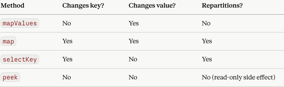
peek is worth a mention, it’s mapValues but returns the value unchanged. Useful for logging or debugging mid-pipeline without affecting the stream:
stream
    .peek((key, value) -> log.info(”Processing: {}”, key))
    .filter(...)
    .mapValues(...);
Windowed aggregation
Without windowing, an aggregation would accumulate forever . your count would just grow from the beginning of time with no useful segmentation. Windows give results meaning by bounding them in time.The key intuition is this: a stream is infinite, but your questions about it aren’t. “How much revenue in the last minute?” has a finite answer: you just need to define which minute. That’s what windows do. They draw a boundary around time so aggregations have somewhere to begin and end.
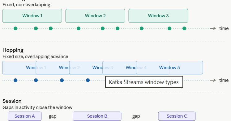
Here’s how the three main window types carve up the same stream of events differently:
Now here’s the complete interactive breakdown of how each window type works in code, with a live simulator showing how events fall into buckets:
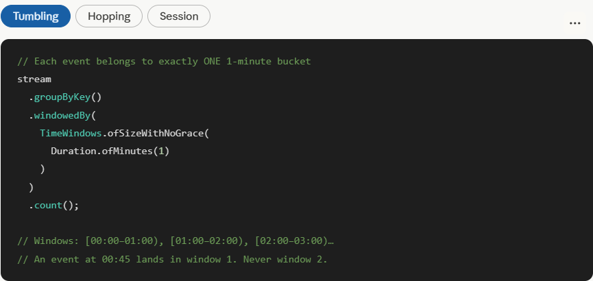
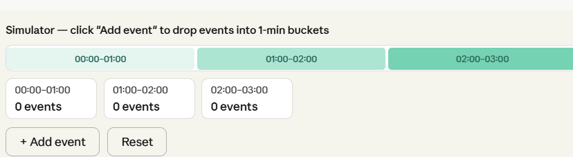
Each event lands in exactly one bucket. No event is ever double-counted. When a window closes, its result is final.
Tumbling windows are the simplest and most memory-efficient. Every event belongs to exactly one bucket, results are final when the window closes, and state stores stay small. Start here unless you have a specific reason not to.
Hopping windows give smoother rolling metrics, because windows overlap, your counts change gradually rather than resetting sharply every minute. The trade-off is memory: each event is stored in multiple windows simultaneously, so state stores grow proportionally to window_size / hop_interval.
Session windows are fundamentally different . They’re driven by behaviour, not the clock. The window size is unknown in advance and varies per key. They’re ideal for modelling real user sessions, but require more careful tuning of the inactivity gap.
One important subtlety — grace periods. All the examples above use withNoGrace, which means a late-arriving event (one whose timestamp is earlier than the current stream time) is simply dropped. In production you almost always want to add a grace period:
TimeWindows.ofSizeAndGrace(
    Duration.ofMinutes(1),   // window size
    Duration.ofSeconds(10)   // accept events up to 10s late
)
This tells Kafka Streams to keep the window open a little longer to accommodate events that arrive slightly out of order, common in distributed systems where network delays are real.
Under the hood, all windowed aggregation state lives in a local RocksDB store on disk, backed by a Kafka changelog topic. If your app restarts, it replays the changelog to restore its state exactly. So your counts survive crashes without reprocessing the entire source topic from the beginning.
A sink topic is the mirror image of a source topic. it’s the Kafka topic your Kafka Streams application writes results to at the end of your processing pipeline.
If the source topic is where raw events come in, the sink topic is where processed, enriched, or aggregated results go out. Other applications — dashboards, databases, microservices, or even another Kafka Streams app can then consume from it.
In the pipeline we’ve been building throughout this conversation, this single line declares the sink:
stats.toStream()
     .map((windowedKey, value) -> new KeyValue<>(windowedKey.key(), value))
     .to(”order-stats”);   // ← this is the sink topic
.to() is the terminal operation. It ends the topology and writes every record to order-stats. Nothing flows further downstream within this app.
Sink topics
You can write to multiple sink topics from one topology. .branch() lets you route different records to different destinationsm, premium orders to one topic, standard orders to another, all within the same app.
This is how you chain Kafka Streams applications into larger pipelines: App A writes enriched orders to enriched-orders, App B reads enriched-orders and writes fraud scores to fraud-scores, and so on. Each app is independently deployable and scalable.
You can also use .through() instead of .to() when you want to write to an intermediate topic and keep processing. .to() is a dead end; .through() writes and hands you back a new KStream to continue working with.
The sink topic is also how Kafka Streams integrates with the rest of your stack. From there, Kafka Connect can pick up the results and push them into Elasticsearch, PostgreSQL, S3, or any other downstream system, without your Streams app needing to know anything about those targets directly.
Kafka Connect
Kafka Connect is the data integration layer of the Kafka ecosystem. It moves data into and out of Kafka without you writing any producer or consumer code. It sits between your sink topics and the outside world.
The core idea is simple: instead of writing bespoke code to push your order-stats topic into PostgreSQL, you configure a connector, a plugin that knows how to talk to a specific system and Connect handles the rest. Polling, batching, retries, offset tracking, scaling, all managed for you.
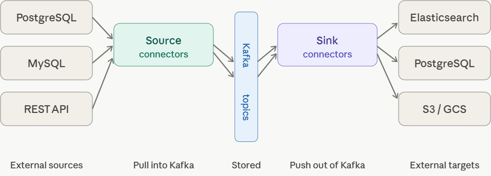
Connect has two connector directions. Source connectors pull data into Kafka from external systems , a database, a REST API, a file system. Sink connectors push data out of Kafka to external targets, Elasticsearch, S3, a data warehouse. Your Kafka Streams sink topic plugs directly into a sink connector.
Configuration, not code
The most important thing about Connect is that you configure connectors with JSON, you rarely write code. Here’s a complete sink connector that takes your order-stats topic and writes every record into Elasticsearch:
{
  “name”: “order-stats-elastic-sink”,
  “config”: {
    “connector.class”: “io.confluent.connect.elasticsearch.ElasticsearchSinkConnector”,
    “tasks.max”: “2”,
    “topics”: “order-stats”,
    “connection.url”: “http://localhost:9200”,
    “type.name”: “_doc”,
    “key.ignore”: “false”,
    “schema.ignore”: “true”
  }
}
You POST that JSON to Connect’s REST API and it starts flowing. No Kafka consumer code, no Elasticsearch client code, Connect handles it all.
Tasks and workers
Under the hood, Connect runs on a cluster of workers (JVM processes). Each connector is broken into one or more tasks, the unit of parallelism. Setting tasks.max: 2 above means Connect will run two parallel tasks pulling from order-stats, each handling a subset of the topic’s partitions. Scale out by adding more workers; Connect rebalances tasks automatically.
Debezium — the source connector worth knowing by name
The most widely used source connector is Debezium, which implements Change Data Capture (CDC). Instead of polling a database with SELECT queries, Debezium tails the database’s binary replication log, the same stream your read replicas use and emits every insert, update, and delete as a Kafka event in real time.
{
  “name”: “postgres-cdc-source”,
  “config”: {
    “connector.class”: “io.debezium.connector.postgresql.PostgresConnector”,
    “database.hostname”: “localhost”,
    “database.port”: “5432”,
    “database.user”: “debezium”,
    “database.password”: “secret”,
    “database.dbname”: “orders”,
    “table.include.list”: “public.orders”,
    “topic.prefix”: “cdc”
  }
}
This emits every change to the orders table as an event on the topic cdc.public.orders — with the full before and after state of the row. Your Kafka Streams app can then consume that topic, joining CDC events with other streams in real time.
How it ties the whole pipeline together
Putting it all together, the full architecture we’ve built across this conversation looks like this:
PostgreSQL (orders table)
  → Debezium source connector
    → order-events topic          ← source topic
      → Kafka Streams app
        (filter → mapValues → aggregate)
          → order-stats topic     ← sink topic
            → Elasticsearch sink connector
              → Elasticsearch (for dashboards)
              → S3 sink connector
                → S3 (for long-term storage)
Every stage is independently scalable, fault-tolerant, and loosely coupled. The Kafka topics act as durable buffers between each layer, if Elasticsearch goes down, records queue up in the sink topic and drain when it recovers, with zero data loss.
Want to go deeper on Debezium and CDC, or explore how Schema Registry keeps the data contracts between all these components consistent?
Apache Kafka Streams is more than just a processing library. It’s a complete rethinking of how applications relate to data in motion.
What started as a deep dive into a single blog post has taken us through the full anatomy of a production-grade streaming pipeline: source topics feeding raw events in, filter and mapValues shaping them as they flow, windowed aggregation turning an infinite stream into meaningful time-bounded metrics, a sink topic carrying results out, and Kafka Connect bridging the gap to every system downstream.
The design philosophy running through all of it is the same: loose coupling through durable, replayable logs. Each component, your Streams app, your Connect connectors, your downstream consumers, can fail, restart, scale, and evolve independently, because Kafka topics act as the resilient buffer between them. That’s not an accident of implementation; it’s the architectural bet Kafka makes, and it pays off at scale in ways that tightly coupled systems simply can’t match.
If you’re building on this for the first time, a practical path forward looks like this: start with a managed Kafka cluster (Confluent Cloud or Amazon MSK) to skip the operational overhead, wire up a simple filter → to() topology to get comfortable with the Streams DSL, then layer in windowed aggregation once your use case demands time-bounded metrics. Add Debezium when you need to react to database changes, and Connect sinks when results need to land in Elasticsearch, S3, or a data warehouse.
The ecosystem around Kafka Schema Registry for data contracts, ksqlDB for SQL-native stream processing, Kafka Connect’s library of 200+ connectors, means you rarely have to solve the integration problem from scratch. The primitives are there. The patterns are proven. The only question left is what you build with them.